Conformal prediction gives you a coverage guarantee that survives any model and any data distribution, and the guarantee is real. On a streaming admission-triage engine for a behavioural-health provider network I asked for 90% and measured 89.5% over 12,000 referrals, which is well inside what the theorem permits and exactly what the model risk committee wanted to see.
The same 12,000 referrals carried 83.2% coverage for patients whose preferred language was neither English nor Spanish, and 55.5% coverage on the tier that means someone needs a face-to-face assessment tonight. Nothing was broken and no assumption was violated, but the guarantee is an average over the population, and an average is silent about the subgroup a fairness audit exists to interrogate. What follows is what that costs to see and what it costs to fix: the arithmetic of per-group calibration, why a bias audit on the ranking says almost nothing about the queue the ranking feeds, why the operating point in the model card was never the operating point, and why the only outcome label available is produced by a clinician who was looking at the score.
Where the score comes from
Referrals reach the network three ways. About 34% arrive from an emergency department with a completed medical clearance, 41% from the crisis contact centre, and the rest from outpatient clinics and self-referral. Volume runs around 214 a day across nine inpatient facilities, one contact centre and 22 outpatient sites. Half of that traffic still speaks HL7 v2, so registration and admission events arrive as ADT messages, A04 on register, A01 on admit, A08 on any subsequent correction, and they land in an HL7v2 store that maps them into FHIR, while the other half writes FHIR directly.
Both converge on one managed FHIR store, and the scorer never polls it. A write
to the store publishes a message to a topic and the scorer subscribes, which is
the part of the
Cloud Healthcare API notification behaviour
worth reading closely before you design around it, because a FHIR notification
carries the resource name in its data field until somebody sets
sendFullResource, and from that moment it can carry personal information, which
the DICOM and HL7v2 notifications never do. The attributes ride along regardless,
and every message has action, resourceType, payloadType, storeName,
lastUpdatedTime and versionId on it, so name-only is not attribute-free and a
subscriber that logs attributes is writing resource types and timestamps into
wherever its logs go. Deletes have a switch of their own,
sendPreviousResourceOnDelete, which puts the whole previous resource on the
wire and which sendFullResource has no bearing on, so ours leaves both off and
the scorer reads back through the API. And a FHIR resource that arrives through a
Cloud Storage import emits no notification at all, although a DICOM import of the
same shape does, which makes FHIR backfills invisible to a streaming consumer: a
fine property once you know it, and an incident when you do not.
The alternative surface is
topic-based subscriptions,
which carry the R5 mechanism back to earlier releases and which you use when the
EHR is the publisher and you cannot put a cloud store in the middle, and since
version 1.1.0 of that guide is built on R4B while shipping a separate R4 package,
the first thing to establish with an integration partner is which of the two they
built against. Historical loads go through
Bulk Data Access, STU 3, whose asynchronous
$export and ndjson output is the only sane way to pull a training corpus
without walking the REST API for a month.
flowchart LR
  V2["ADT v2 feed<br/>A01 / A04 / A08"] --> HS[HL7v2 store]
  EHR["EHR FHIR writes"] --> FS[(FHIR store)]
  HS --> FS
  FS -->|Pub/Sub notification| SC{{"Triage scorer"}}
  SC --> TB["Tabular: XGBoost over<br/>Observation, Condition, Encounter"]
  SC --> IM["Imaging: ResNet-50 on the<br/>clearance study, 34% of arrivals"]
  SC --> NR["Narrative: LLM extractor<br/>over DocumentReference"]
  TB --> CF["Conformal set over<br/>ServiceRequest.priority"]
  IM --> CF
  NR --> CF
  CF --> RA["RiskAssessment<br/>written back"]
  CF --> CD["CDS Hooks card"]
  CD -->|"/feedback"| FB["accepted | overridden"]
  style CF fill:#0f766e22,stroke:#0f766e,stroke-width:2px
  style FB fill:#f59e0b22,stroke:#b45309
Three channels feed one score. Gradient boosting over 250 tabular features drawn
from Encounter, Condition, prior utilisation and instrument scores, the last
of which arrive as Observation resources under the
US Core screening-assessment profile, whose
screening and assessments guidance
names PHQ-9 directly and works a full example through it. C-SSRS is not in that guidance, so those
items arrive as plain observations against a local code and the mapping is ours
to maintain. A ResNet-50 backbone over the medical
clearance study, which exists only for the third of referrals routed through an
emergency department, so the imaging features are NaN for everyone else and
gradient boosting handles the absence natively instead of imputing a fiction. And
a language model over the referral narrative in DocumentReference, extracting a
fixed schema of risk markers: means access, housing instability, substance
co-use, prior attempt, current supports.
The narrative channel never leaves the boundary, so the extractor runs inside the same project as the store, the feature vector that reaches the ranker carries integers and booleans and no free text, and the audit record keeps resource references instead of copies, which is the choice that makes the de-identification story tractable later, because a record that quotes a clinical note has to be treated as the note.
The model emits a distribution over the four values of ServiceRequest.priority,
routine, urgent, asap and stat, and the label is that same field adjudicated at
72 hours by a clinician who never saw the score, which makes it a retrospective
judgement of what priority the referral warranted rather than a reading of how
the patient is doing at hour 72. The adjudicator is blind to the score, though
they are not blind to the chart, and the last section is about what that costs.
Getting that adjudication set up was the single most expensive thing in the
project and I would spend the money again, because the alternative label everyone
reaches for first is what happened next in the system, and what happened next in
the system is what the system decided. Obermeyer and colleagues published the
canonical version of that mistake in
Science in 2019: an algorithm trained
on health care costs instead of illness, where remedying the resulting disparity
moved the share of Black patients above the programme’s 97th-percentile
auto-identification threshold from 17.7% to 46.5%, two numbers that belong to
that threshold and move with it. Cost measured who had already been able to spend
on care, so the model learned access and reported it as need. Our adjudication
window is 72 hours because that is roughly how long it takes for a chart to carry
enough to judge from, and the blinding rule, the window and the sampling rate all
sit in the same protocol document.
What a coverage guarantee is a promise about
Split conformal prediction is four lines. Score every calibration point by how
badly the model treated its true label, take a quantile of those scores, and emit
every label whose score falls under it. The quantile is not the empirical
1 - alpha quantile, and the correction matters at small sample sizes:
Angelopoulos and Bates state it as the
ceil((n+1)(1-alpha))/n quantile, and their equation 1 gives the two-sided
result.
import numpy as np

TIERS = ["routine", "urgent", "asap", "stat"]      # ServiceRequest.priority

def conformal_quantile(scores: np.ndarray, alpha: float) -> float:
    """The (1-alpha) split-conformal threshold, with the finite-sample correction.

    Returns inf when the group is too small for the level to exist, which is
    n < ceil(1/alpha) - 1. That is not an error: the prediction set becomes the
    whole tier list, which is a valid interval and a useless one.
    """
    n = len(scores)
    k = np.ceil((n + 1) * (1 - alpha))
    if k > n:
        return np.inf
    return float(np.sort(scores)[int(k) - 1])          # the k-th smallest, exactly

def calibrate(probs: np.ndarray, y: np.ndarray, alpha: float, groups=None):
    """One quantile if groups is None, otherwise one per group."""
    scores = 1.0 - probs[np.arange(len(y)), y]        # least-ambiguous-set score
    if groups is None:
        return {None: conformal_quantile(scores, alpha)}
    return {g: conformal_quantile(scores[groups == g], alpha)
            for g in np.unique(groups)}

def predict_set(probs: np.ndarray, qhat: float) -> np.ndarray:
    return (1.0 - probs) <= qhat
Two details in there are worth more than the rest of the function. The theorem
names a specific order statistic, the k-th smallest calibration score with
k = ceil((n+1)(1-alpha)), so what the code owes it is that element and not a
weighted blend of two, which is why the line sorts and indexes instead of asking
for a quantile. np.quantile(scores, k/n, method="higher") is what I shipped
first and it returns the k+1-th, so at n = 4,000 it hands back the 3,602nd score
where the proof asks for the 3,601st, and switching to method="inverted_cdf" at
the same level fixes almost all of it and not all of it, because k/n is a float
and n * (k/n) lands a hair above k for 92 of the 19,992 group sizes between 9
and 20,000, at which point it rounds up and you are back on the k+1-th score.
None of our own cell sizes is one of the 92, which is why no number in this post
moved when I changed the line. Both versions are conservative and neither is
invalid, but neither is the threshold the theorem is about. Above n = 18 the
error is always exactly one order statistic, a larger move in score the smaller
the group, and at or below 18 it disappears altogether, because ceil((n+1)·0.9)
equals n there and every method returns the largest calibration score.
The infinity branch is the other one, and it fires on real cells. The level
exists only when ceil((n+1)(1-alpha)) <= n, which rearranges to
n >= ceil(1/alpha) - 1, so at alpha 0.10 a group needs nine calibration points
before the procedure can say anything narrower than “one of these four tiers”,
and below that it still satisfies the guarantee, by abstaining from saying
anything at all.
On a calibration set of 4,000 referrals at alpha 0.10 the threshold came out at 0.8377 and the realized coverage on the next 12,000 was 89.50%, which is below the nominal 90% and correct, since coverage conditional on the calibration draw is itself a random variable, Beta(n+1-l, l) with l = floor((n+1)·alpha), which Angelopoulos and Bates give in their section 3.2 and credit to Vovk. For these numbers that is Beta(3601, 400): mean 90.00%, standard deviation 0.47 points, fifth percentile 89.21%, so a realized 89.50% sits just under the fifteenth percentile of that law. The guarantee is over draws of the calibration set, and you get one draw. Set sizes came out at 20.7% singletons, 45.5% spanning two tiers, 32.0% spanning three and 1.7% spanning all four, for a mean of 2.15 tiers out of four, and nobody in the clinical governance meeting cared about the coverage number, but they cared a great deal that a third of referrals came back with three tiers highlighted, because a card that says “urgent or asap or stat” is a card that has told a charge nurse nothing she did not know.
The axis the audit is about
The network’s fairness review is organised around preferred language, and it is worth being precise about why, because the regulation does not say what people in the room kept saying it says. 45 CFR 92.210 is short and has three parts. Subsection (a) forbids a covered entity to discriminate through the use of patient care decision support tools on the basis of race, colour, national origin, sex, age or disability, subsection (b) requires reasonable efforts to identify tools that employ input variables measuring those characteristics, and (c) requires reasonable efforts to mitigate the resulting risk. Language is not in that list, and preferred language and limited English proficiency are handled a section earlier, in §92.201, which is about meaningful access and says nothing about decision support.
So the identification duty in (b) does not reach this model on its face, since nothing in it takes language as an input and language is not one of the enumerated characteristics anyway, and what does reach it is (a), whose prohibition is not conditioned on the input list at all. We chose preferred language as the audit axis because it is the recorded field in our data that sits closest to national origin and because a tool can discriminate on a basis it never ingests, which is a design judgement about a proxy, and we wrote it into the model card as one and not as a citation.
That argument survives right up to the point where the fix ships. The group-conditional calibration two sections down puts a separate threshold on each language group, and the card the clinician reads says the set was calibrated within this patient’s language group, so language is an input to the deployed output even though the ranker never sees it. Set that next to the sentence about choosing language for its closeness to national origin and the identification duty in (b) has an argument it did not have before, assembled out of our own model card. It may still not bite, since (b) is scoped to input variables measuring the listed characteristics and language is not one of them, but we stopped relying on that, and the coverage partition is now reported under (b) as though the duty applied, which costs a paragraph and removes the need to win the point.
Coverage by language group, from the same pooled quantile that produced 89.50% overall: English 90.72% on 9,410 referrals, Spanish 86.10% on 1,655, everything else 83.21% on 935. Those weight back to 89.50% exactly, which is an identity and not a finding, since the marginal number is defined as their size-weighted mean and would reconcile at any coverage at all, and the guarantee is about that weighted average, on which none of the three groups is sitting.
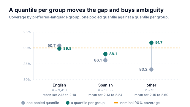
The teal dots in that figure are the fix, and I will get to what they cost two sections down. The short version is under the last pair: bringing the smallest group from 83.21% to 91.66% coverage widens its mean prediction set from 2.15 tiers to 2.60 out of four.
The mechanism is not mysterious and it is not a bias in the ordinary sense. When a crisis call runs through an interpreter it takes longer per unit of content and the note that results is shorter, so the LLM extractor recovers fewer risk markers, so the tabular vector for those referrals carries less signal, so the model’s probabilities are closer to noise while still occupying the full range, and AUC on the escalation head reflects the whole chain: 0.860 for English, 0.795 for Spanish, 0.771 for the rest, against 0.844 pooled. A model that is genuinely less certain about a group should produce wider sets for that group, and one pooled quantile is perfectly capable of doing so, since set width still depends on where a group’s own probabilities sit relative to the threshold, but nothing in the procedure makes it produce enough of it. The threshold is fitted to the population’s score distribution and the population is 78% English, so it lands where the majority puts it and the smaller groups absorb the difference as missed coverage instead of as width.
Lei, G’Sell, Rinaldo, Tibshirani and Wasserman put the distinction in a remark that deserves to be printed and stuck to a wall: the probability statements are taken over the samples, so they assert average coverage, and this should not be confused with coverage conditional on the covariates, which is a much stronger property. Angelopoulos and Bates give the same point as a two-group example where the sets always cover one group and never cover the other and the marginal number is still 90%.
Before any of that, though, the check that failed to catch it. The calibration dashboard the governance committee reads is expected calibration error, ten deciles of the score, and it read 0.0100 across the population, where per group, on the same bin edges, it read English 0.0186, Spanish 0.0288, other languages 0.0454. The pooled number is smaller than every single group inside it, and that is not an accident of this dataset: inside a bin, the pooled deviation is a weighted average of the group deviations, the absolute value of a weighted average is at most the weighted average of the absolute values, and summing that over bins gives pooled ECE at most the size-weighted mean of the group ECEs, which is in turn at most the worst group’s. On shared bin edges the inequality is a theorem and it always points the same way, with cancellation making it strict rather than tight: inside the top decile, mean predicted risk was 0.670 against observed rates of 0.714, 0.592 and 0.576 by group, and 0.688 pooled, so the deviations point in opposite directions and most of the error disappears. The consequence for the dashboard is the part that matters, because a low pooled ECE is not evidence that any group is calibrated, whereas a high one does prove some group is at least that bad, and the committee was reading the metric in the only direction it cannot be read. It took me most of a quarter to stop doing the same.
Recalibrating the pooled probabilities did nothing at all, and I want to record that as the null result it was. Brier score on the escalation head: 0.11942 raw, 0.11941 with Platt scaling, 0.11950 with isotonic regression, over three runs on one evaluation set, with no difference I could distinguish from the third decimal place. The model was already calibrated in the pooled sense, so there was nothing there for a pooled recalibration to fix, and neither fitted calibrator went into the pipeline.
from sklearn.calibration import CalibratedClassifierCV
from sklearn.frozen import FrozenEstimator

# cv="prefit" is deprecated in scikit-learn 1.6 and is removed in 1.8; the
# wrapper is now the supported way to calibrate an already-fitted estimator.
platt = CalibratedClassifierCV(FrozenEstimator(base), method="sigmoid").fit(Xc, yc)
iso   = CalibratedClassifierCV(FrozenEstimator(base), method="isotonic").fit(Xc, yc)
The tier where it fails is the tier that matters
Language is one conditioning axis, but the label is another and it is worse.
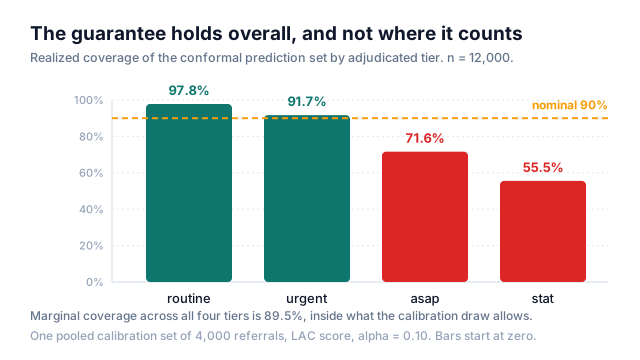
Coverage on routine referrals was 97.82%, on urgent 91.68%, on asap 71.60% and on stat 55.54%. Turn that last figure around and it is the sentence that ended the meeting: 44.46% of the referrals that genuinely warranted an immediate assessment came back with a prediction set that did not contain that tier. Routine referrals are 52% of traffic at 97.82% coverage, so they put 0.510 of the 0.895 marginal on the board by themselves, while stat is 7.4% of traffic at 55.54% and contributes 0.041.
This is a property of the score I chose, because the least-ambiguous-set score minimises average set size and buys that efficiency by spending errors on rare classes. If you want a score that adapts its width to the difficulty of the input, the literature to read is Romano, Sesia and Candès, whose section 2.4 sets out the complaint against homogeneous conformal classification: one threshold gets applied to the easy inputs, where a single label already holds almost all the probability, and to the hard ones, where the probabilities sit near one over the number of classes, so the coverage those two regions actually receive comes out unequal. The four coverage figures above are that same phenomenon measured along the label instead of along the input, one threshold reading 97.82% where the model is rarely wrong and 55.54% where it usually is, and the adaptive score their paper proposes exists to approximate the conditional coverage that would close both kinds of gap. Their motivating oracle construction in section 1.1 can return the empty set, which is worth knowing before you switch scores, because an empty set renders as no card at all and a queue reads no card as no risk.
With LAC the arithmetic is simpler than I assumed for a year, since the largest of four probabilities is always at least 0.25, so a single threshold produces an empty set only when it falls below 1 - 1/K, which is 0.75 here, and at exactly 0.75 the set still has a member. Ours was 0.8377, and the three group thresholds in the next section are 0.8293, 0.8594 and 0.9079, all clear of it, though a threshold of 0.72 would have produced empty sets silently and the rendering path would not have noticed. That test stops applying the moment there is a threshold per tier, since the routine threshold in the fix below is 0.6915, and what carries the per-tier version is a different sum: the four values of one minus the threshold come to 0.610 while the four probabilities come to 1, so at least one tier always clears its own bar.
The direct fix is a quantile per tier, which is Mondrian conformal prediction applied to the label, a name that comes from a 2003 construction of Vovk and colleagues by way of the painter’s grids, and which means cutting the calibration set into cells and taking a separate quantile inside each. It works, and it works hard: coverage on stat moved from 55.54% to 91.60% and on asap from 71.60% to 93.10%. It costs the thing you were buying, though, because the mean set went from 2.15 tiers to 2.45 and 11.8% of all referrals came back with every tier highlighted. It barely touched the language axis either, where the three groups went to 91.39%, 86.40% and 84.17%, each up between 0.30 and 0.96 points on the pooled numbers, and the marginal rose to 90.14%, while the spread between the best and worst group went from 7.51 points to 7.22. Conditioning on one variable lifts the others a little and closes nothing, because it makes no statement about them at all. Both fixes were on the table at the same governance meeting, and the question of which one to spend the calibration set on turned out to be the whole design decision.
What conditioning costs in labelled points
Group-conditional coverage is achievable. The construction is old, and the
statement I calibrate against, because it carries the explicit upper bound, is
Romano, Barber, Sabatti and Candès on equalized coverage,
whose own paper credits five earlier sources for variants of the lemma it rests
on. Calibrate separately inside each group and you get coverage at least
1 - alpha within every group, and, where that group’s conformity scores are
almost surely distinct, an upper bound of 1 - alpha + 1/(|I2(a)| + 1) as well,
with |I2(a)| the group’s calibration count. The distinctness condition attaches
to the upper bound alone; the lower one holds without it, and ties in the score
are what would cost you the upper one. The whole cost of the method is in that
denominator.
from crepes import WrapClassifier
from sklearn.ensemble import RandomForestClassifier

def language_bin(X):
    """One Mondrian category per row: the declared audit attribute itself."""
    return X[:, 3].astype(int)                # 0 = en, 1 = es, 2 = other

model = WrapClassifier(RandomForestClassifier(n_estimators=200, random_state=0))
model.fit(Xtr, ytr)
model.calibrate(Xc, yc, mc=language_bin, seed=0)   # mc, not class_cond
sets = model.predict_set(Xt, confidence=0.90, labels=False,
                         smoothing=False, seed=0)   # int64 (n, 4), not bool
Three things in nine lines cost me an afternoon each. mc= takes either a
MondrianCategorizer or a plain callable, and only the callable does what you
probably want: calibrate runs bins = mc(X) and uses the returned values as
categories directly. Hand it a MondrianCategorizer fitted with
fit(X=Xc, f=..., no_bins=k) instead and it will call binning(f(X), bins=k),
which treats your function’s output as a score and cuts it into k
equal-frequency bins. On my language mix that splits English across two bins and
lumps Spanish and other together, which is a partition, but not the one I asked
for and not one anybody would notice from the output.
The second is that the two Mondrian axes do not compose. class_cond=True
conditions on the label and is what fixed the stat tier above; mc= conditions
on anything you can compute from a row. Pass both and calibrate takes the
class_cond branch and never looks at mc again, silently. Crossing the two
axes means building the crossed categoriser yourself, which is exactly why the
twelve-cell table below is the shape of the problem rather than a footnote to it.
The third is smoothing, which defaults to True. Leave it and you are running
randomized conformal prediction, a different procedure with a different set-size
distribution from the one described in every paragraph above. Also
predict_set(labels=False) returns an int64 indicator matrix rather than a
boolean one, which matters the moment you index with it.
Per language group my calibration set of 4,000 split 3,128 / 580 / 292, giving
thresholds of 0.8293, 0.8594 and 0.9079 and coverage of 89.80%, 88.10% and
91.66%. The spread between the best and the worst group falls from 7.51 points to
3.56, and Spanish comes in 1.90 points under nominal on a 580-point cell whose
realized coverage has a standard deviation of 1.24 points. The 91.66% is worth a second look, because two
paragraphs ago the upper bound for a 292-point group was
1 - alpha + 1/293, or 90.34%, and 91.66% is above it. The bound is on the
probability marginalised over draws of the calibration set, not on the number one
draw produces, and under Beta(264, 29) a realized 91.66% sits at the 81st
percentile, so nothing is violated. The fifth percentile of that same law is 87.09%,
against 89.21% for the pooled set, so the guarantee I just bought for the
smallest group has 3.7 times the standard deviation of the one I gave up.
Now cross the two axes, because the question a clinical safety officer actually asks is whether the stat tier is covered for the smallest language group. Twelve cells, 4,000 calibration points, and the arithmetic is brutal at the corner.
| calibration cell | n | Beta | sd of realized coverage | 5th percentile | upper slack |
|---|---|---|---|---|---|
| English, routine | 1,638 | Beta(1476, 163) | 0.74 pts | 88.81% | +0.06 pts |
| English, stat | 228 | Beta(207, 22) | 1.94 pts | 87.01% | +0.44 pts |
| Spanish, urgent | 166 | Beta(151, 16) | 2.27 pts | 86.43% | +0.60 pts |
| Spanish, asap | 94 | Beta(86, 9) | 2.99 pts | 85.17% | +1.05 pts |
| Spanish, stat | 23 | Beta(22, 2) | 5.53 pts | 80.98% | +4.17 pts |
| other, asap | 44 | Beta(41, 4) | 4.20 pts | 83.31% | +2.22 pts |
| other, stat | 27 | Beta(26, 2) | 4.78 pts | 83.60% | +3.57 pts |
Seven of the twelve cells are shown; the five omitted ones carry 852, 410, 297, 136 and 85 points. Counts come from one contiguous calibration window of 4,000 consecutive referrals, which is about nineteen days at 214 a day, and the twelve cells sum to 4,000 exactly.
Twenty-three calibration points is above the nine the level needs, so the procedure runs and reports a number. That number, however, has a standard deviation of 5.5 points and a one-in-eight chance of landing under 85%. Angelopoulos and Bates give the sizing directly in their Table 1: to hold the coverage slack inside plus or minus 0.05 with 90% confidence you need 102 calibration points, and inside plus or minus 0.01 you need 2,491, per cell rather than in total. To guarantee the corner of that table to a point you would need more calibration data in one cell than the whole model was trained on.
Now read the last two rows against each other, because this is the part I had
backwards for two quarters. The other, asap cell has 44 calibration points and
a fifth percentile of 83.31%. The other, stat cell has 27, and its fifth
percentile is 83.60%. Fewer labelled points, better worst case, in adjacent rows
of the same table. That is not rounding and it is not a quirk of these counts.
The fifth percentile of Beta(n+1-l, l) is not monotone in n, because
l = floor((n+1)·alpha) steps up by one whenever (n+1)·alpha crosses an
integer, which at alpha 0.10 is n = 19, 29, 39 and every tenth value after.
Eighteen calibration points give a fifth percentile of 84.67%, and nineteen give
77.36%.
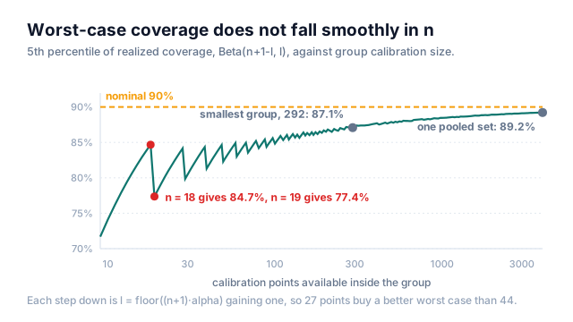
One additional labelled referral, 7.31 points of worst-case coverage gone, and then a climb back. The climb more than repays the step: over the ten points from 19 to 29 the curve nets 2.48 points up, and every cycle after that nets up as well, by 1.46 from 29 to 39 and 0.98 from 39 to 49, so between 9 and 129 points there are exactly two cell sizes at which ten more labels leave the worst case lower than it started, n = 27 and n = 28. The version that caught me is wider than a single step, because a cell of 18 points has a better fifth percentile than every cell size from 19 through 57, so on that stretch forty more labelled referrals buy nothing at all, and the two rows in the table are that same effect seen over a seventeen-point gap that crosses two steps.
The practical consequence is that two of the sentences I had been saying in governance meetings were wrong. “More calibration data is better” is true in the limit and false locally, and “this cell has more points than that one, so trust it more” is not an argument at all in the range where the small cells live. What you compare between cells is the fifth percentile itself, which is why the model card carries that column and the count is only there to explain it.
The uncomfortable half of this is that it invites a move I haven’t been able to talk myself into. If the worst case at 18 points beats the worst case at every size up to 57, and a cell is sitting at 40, then discarding calibration points to land on 18 improves the number the model card reports. The arithmetic is sound but the instinct that it is cheating is also sound, and I have never satisfied myself about which one wins. Throwing away labelled data to make a bound look better is obviously the wrong shape of act, but the bound is not a rhetorical device, it is the quantity a safety argument rests on, and a procedure run at 18 points genuinely does have a better fifth percentile than the same procedure run at 40. My working position is that the choice of cell size has to be made before the calibration window opens and recorded with the audit partition, which converts the question from a data-handling decision into a design one and stops anybody making it after seeing the outcome. That is a governance answer to a statistical question and I know it. Nobody I asked had a better one, and the literature I could find treats n as given rather than as chosen, which is a reasonable thing for a paper to assume and an unreasonable thing for an operator to inherit.
There is no trick that avoids this, and the reason is a theorem rather than an
engineering gap. Asking for coverage conditional on the covariates, exactly and
without distributional assumptions, forces the procedure to return an interval of
infinite expected length at almost every non-atomic point.
Barber, Candès, Ramdas and Tibshirani give
that as Proposition 1, and their own header credits it to Vovk in 2012 and to
Lei and Wasserman in 2014, so exact conditional coverage and informative output
cannot be had together. Their Theorem 3 is the version
you can actually build, and it is the one that shaped the design. Coverage
restricted to a class of sets you specify in advance is achievable, and only for
the members of that class carrying at least a stated share delta of the
population. Their own worked reading of it is that at
delta = 0.10 the promise covers any subgroup making up a tenth of traffic. That
second half is what the table above runs into. The Spanish, stat cell is 23
calibration points out of 4,000, six-tenths of one percent, so it sits under any
delta a committee would write down and the theorem never offered it anything.
So the audit
groups became a governed artifact, declared before calibration, versioned, and
changed only through the model risk committee. Adding a group after the fact is
not a reporting change but a new calibration set and a new validation.
Choosing that list is a clinical conversation and not a statistical one. Our medical director wanted adolescent status in the partition, since the whole pathway differs for under-18s, and adding it took the smallest cell under 20 points. We kept language and age band as two independent partitions and never crossed them, reported both marginally within their own axis, and wrote into the model card that no joint cell carries a guarantee. That sentence took three weeks to agree, most of it spent on whether a regulator would read “no guarantee” as an admission, and it survived because the alternative was a number none of us could have defended if asked how it was computed.
Where the ranking gets cut
Everything above is about the score, but the system is a queue.
The ranking-level audit is what goes on the model card: AUC 0.844 pooled, 0.860 for English, 0.795 for Spanish, 0.771 for the rest, a gap that was noted and accepted with a monitoring commitment. What the committee did not have in front of it is that the disparity a patient experiences is not a property of the ordering. It is a property of where the ordering gets cut, and the cut is set by how many structured assessments the rota can supply.
from fairlearn.metrics import MetricFrame

def true_positive_rate(y_true, y_pred):
    pos = y_true == 1
    return float(y_pred[pos].mean())

mf = MetricFrame(metrics={"tpr": true_positive_rate},
                 y_true=esc, y_pred=flagged, sensitive_features=lang,
                 n_boot=1000, ci_quantiles=[0.025, 0.975], random_state=0)
lo, hi = mf.by_group_ci               # a list of frames, one per quantile
print(mf.by_group, mf.ratio())
MetricFrame is keyword-only throughout, and by_group_ci returns a list of
frames in the order of ci_quantiles instead of a frame with interval columns,
which is the kind of shape you find out about by unpacking it wrong. The
intervals earn their place here: at the published threshold the true positive
rate was 0.8438 for English, 0.7341 for Spanish and 0.6990 for the rest, and the
95% bootstrap interval on that last one runs [0.6349, 0.7598] on 935 referrals.
A subgroup metric quoted without an interval is a number about 935 people
pretending to be a number about the model.
Then vary the cut.
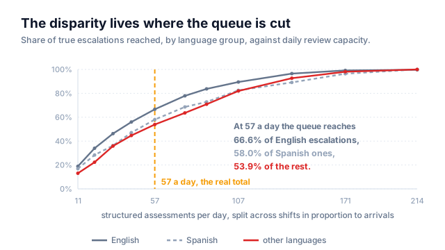
That curve splits each day’s capacity across the three shifts in proportion to arrivals, which is the allocation you would design on paper. At 57 a day it reaches 66.6% of the English-language patients who needed escalating, 58.0% of the Spanish-language ones and 53.9% of everyone else. The rota the network actually works is 26 slots on days, 20 on evenings and 11 overnight, and running the same 57 assessments through it gives 66.3%, 55.9% and 54.9%. Two things fall out of this and both of them matter more than the AUC gap.
The absolute equal-opportunity gap is not monotone in capacity, and it is not smoothly non-monotone either. It runs 0.058 at 11 reviews a day, 0.117 at 21, back down to 0.104 at 32, up through 0.114 and 0.127 to a peak of 0.143 at 75, then down to 0.075 at 107 and 0.003 at 214. The local maximum at 21 and the dip at 32 are one draw of a ranking against one set of cut points and I would not read anything into either, whereas the shape of the whole curve is forced. Every group’s true positive rate is zero when nobody is reviewed and one when everybody is, so the gap is pinned to zero at both ends and does its damage in the middle, which is where every real system operates. An equal-opportunity number quoted without the review depth it was computed at is not a measurement.
The other is that the four-fifths ratio moves under both levers, and the whole range in play sits within a few points of 0.80. Neither §92.210 nor the decision-support criterion at 170.315(b)(11) makes that number a threshold, and it is worth saying so plainly. Four-fifths is a convention out of the Uniform Guidelines on Employee Selection Procedures, scoped to employment, hedged even there, and our committee had adopted it because it wanted a line and not because a regulation supplied one. It is still the number that gets read out. On the proportional split the min-max true positive ratio is 0.797 at 43 reviews a day and 0.809 at 57, so under that one allocation the 0.80 line is crossed between two staffing levels the network has actually run in a bad month. Both of those figures belong to the proportional split and not to the rota. Hold the total at 57 and change only how the slots are spread across shifts and the same model on the same population reads 0.828, which is the number our audit would have reported. Where the real rota crosses 0.80 we have never computed, because the crossing belongs to an allocation and we only ever measure one allocation at a time. Neither number is the model’s and neither is stable, whereas both would be reported as a property of the model. The prohibition in §92.210 lands on the covered entity, and the covered entity’s ML team does not set the rota. What we do now is compute the ratio at the rolling four-week realized capacity and shift allocation, and carry it into the monthly operations review alongside vacancy rates. The line names the allocation it was computed under, and it gets reissued when the rota changes.
The rota sets the operating point
The model card publishes precision at fixed recall, which is the convention, and the convention hides a category error.
The threshold was fitted on the calibration split for recall 0.80. On the evaluation set it produced recall 0.8173 at precision 0.4195, which is admissible against the ceiling of 2,502 positives over 4,875 flags, or 0.5132. It also flags 87.1 referrals a day. The clinicians review 57.
| shift | arrivals | flagged at threshold | capacity | realized recall | realized precision |
|---|---|---|---|---|---|
| day | 88.5 | 35.7 | 26 | 0.6815 | 0.4718 |
| evening | 80.8 | 33.1 | 20 | 0.6162 | 0.5232 |
| night | 45.0 | 18.4 | 11 | 0.6022 | 0.5308 |
| network | 214.3 | 87.2 | 57 | 0.6395 | 0.5013 |
Eight weeks of production traffic, 12,000 referrals, one adjudication pass at 72 hours. Arrival and flag counts are per shift and per day respectively.
Recall 0.80 was never delivered on any shift. What the network actually runs at is 0.6395, while precision moves the other way and comes out better than published, at 0.5013, because truncating a ranked list from the bottom removes the weakest flags, so both numbers move by shift, they move in opposite directions, and no single summary of the pair is stable across a rota. I stopped reporting precision at fixed recall and started reporting both at fixed capacity, with capacity as an explicit input the staffing office signs off on alongside the model. Reporting it that way changed the conversation immediately, because the nursing leads had been asked to react to a model’s operating point for a year, and once the operating point was visibly theirs, the evening shift argued for four more slots and got them. The model card now carries both pairs, nominal and realized, each labelled with the capacity it was computed at.
The only label you have was produced by someone looking at the score
The card fires whenever the prediction set touches asap or stat, which is 38.3% of referrals.
SYS = "http://example.org/triage-override"
OVERRIDE_REASONS = [                    # ordered by expected frequency, not alphabetically
    {"code": "no-bed", "system": SYS, "display": "No appropriate bed in network"},
    {"code": "lower-acuity", "system": SYS, "display": "Assessed at a lower acuity"},
    {"code": "already-engaged", "system": SYS, "display": "Already under active care"},
    {"code": "insufficient-record", "system": SYS, "display": "Referral record too thin"},
    {"code": "patient-declined", "system": SYS, "display": "Patient declined the pathway"},
]

def triage_card(prediction_set, encounter_id, card_uuid):
    """A CDS Hooks 2.0 card. Fires only when the set touches an escalation tier."""
    idx = [i for i, inc in enumerate(prediction_set) if inc]
    tiers = [TIERS[i] for i in idx]
    if not ({"asap", "stat"} & set(tiers)):
        return None
    indicator = "critical" if "stat" in tiers else "warning"
    contiguous = idx == list(range(idx[0], idx[-1] + 1))   # {routine, stat} is not
    span = (tiers[0] if len(tiers) == 1
            else f"{tiers[0]} to {tiers[-1]}" if contiguous
            else " or ".join(tiers))
    return {
        "uuid": card_uuid,
        "summary": f"Triage model: priority {span}",
        "indicator": indicator,
        "detail": ("90% prediction set at alpha 0.10, calibrated within this "
                   "patient's language group. Set width is the model's "
                   "uncertainty, not the patient's severity."),
        "source": {"label": "Admission triage model v4.2",
                   "url": "https://internal/model-cards/triage-4-2"},
        "selectionBehavior": "at-most-one",
        "suggestions": [{                        # without this, no feedback row
            "label": "Book a structured assessment within the shift",
            "uuid": f"{card_uuid}-assess",
            "actions": [{
                "type": "create",
                "description": "Assessment request at the set's top tier",
                "resource": {"resourceType": "ServiceRequest",
                             "status": "draft", "intent": "plan",
                             "priority": tiers[-1],       # raises, never lowers
                             "encounter": {"reference": f"Encounter/{encounter_id}"}},
            }],
        }],
        "overrideReasons": OVERRIDE_REASONS,
        "links": [{"label": "Score provenance", "type": "absolute",
                   "url": f"https://internal/triage/{encounter_id}"}],
    }
CDS Hooks 2.0 is unusually well designed for
this problem, and overrideReasons is the reason. A card can ship a coded list
of reasons a clinician may pick when declining it, and the feedback endpoint at
/cds-services/{id}/feedback takes them back with an outcome of accepted or
overridden, an overrideReason.reason coding and a free-text userComment.
Structured dissent, delivered by the standard, at no cost beyond writing the
value set.
The suggestions array is not decoration, and shipping without it is what my
first version did. An outcome of accepted in the feedback payload means the
user took one or more suggestions, and the payload carries their identifiers in
acceptedSuggestions. A card with no suggestions can therefore only ever come
back overridden or not come back at all, which makes the acceptance rate
undefined rather than zero. Everything in the rest of this section rests on the
accepted arm existing, so it is worth checking against the spec before you
measure anything on it.
def ingest_feedback(body: dict) -> list[dict]:
    """POST /cds-services/{id}/feedback. Every row is a label with a caveat."""
    rows = []
    for fb in body["feedback"]:
        reason = (fb.get("overrideReason") or {}).get("reason") or {}
        rows.append({
            "card_uuid": fb["card"],
            "outcome": fb["outcome"],                     # accepted | overridden
            "accepted": [s["id"] for s in fb.get("acceptedSuggestions", [])],
            "override_code": reason.get("code"),
            "user_comment": (fb.get("overrideReason") or {}).get("userComment"),
            "at": fb["outcomeTimestamp"],
            # the two fields that decide whether this row may enter a metric
            "card_shown": True,
            "score_visible_to_reviewer": True,
        })
    return rows
Overrides ran at 30.02%, and broken down the pattern is legible and none of it is
about whether the model was right. Cards carrying the critical indicator were
overridden 13.94% of the time and warning cards 37.69%. Cards whose prediction
set spanned three or four tiers were overridden 32.13% of the time against 14.42%
for narrow sets, so within a group, width predicts decline: a wider set is less
actionable and a less actionable card gets waved away.
Width does not explain the language split, though, and I spent a while assuming
it would. English cards were overridden 28.30% of the time, Spanish 36.38% and
other languages 35.90%. Under the pooled quantile that produced these cards the
three groups have almost identical mean set sizes, 2.15, 2.13 and 2.15. One
threshold can happily hand one group wider sets than another, since width follows
each group’s own score distribution and not the threshold on its own, but on this
data it did not, which is why the pooled quantile shows up in the coverage
numbers and stays invisible in the widths. Whatever drives the seven-point spread
between English and Spanish is not set width, and I have not measured what it is. What I can say, however, is which direction the fix
pushes. The
group-conditional calibration two sections up widens other from 2.15 tiers to
2.60, which lands the width penalty on one of the two groups already declining
the most cards. Equalising coverage and reducing overrides are not the same
project, and here they pull against each other.
The temptation is to treat the override stream as ground truth, because it is free, structured and arrives in real time, but against the 72-hour adjudication it does not survive contact.
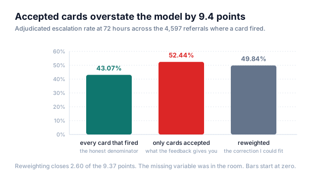
Across all 4,597 fired cards the adjudicated escalation rate was 43.07%, and across the cards a clinician accepted it was 52.44%. Scoring the model on its accepted cards, which is what every dashboard I inherited was doing, overstates it by 9.37 points, and the mechanism is not subtle: clinicians decline the cards the model got wrong, which is them doing their job and me losing my denominator.
I fitted an inverse-probability model to recover the missing cases, on everything the system could observe at the moment of the card: score, indicator, set width, language group. It closed 2.60 points, with a 95% bootstrap interval over 3,000 resamples of [2.29, 2.90], and left 6.77 points on the table. The residual is not a modelling failure I can fix by adding features, because the variable driving the override is the part of the patient’s presentation the clinician saw in the room and the referral record never carried. A propensity model built only from what the model saw cannot recover a selection driven by what the model did not see. So the override stream became a monitoring signal with a stated bias, and the 72-hour adjudication that covered all 12,000 referrals for this measurement kept running afterwards on a stratified 15% sample, stratified by language group and shift so the small cells do not thin out.
The system erodes the label it was trained on
The last thing that moved was the label, and it moved without anything else moving.
| quarter | top-decile precision | max feature PSI |
|---|---|---|
| Q1 | 0.693 | 0.041 |
| Q2 | 0.654 | 0.058 |
| Q3 | 0.670 | 0.049 |
| Q4 | 0.611 | 0.072 |
Reviewed top decile is 21 assessments a day, 9.8% of arrivals. PSI is the maximum across 16 monitored features, computed weekly against the training window and reported here as the quarterly maximum. Four quarters, one model version, no retraining.
Precision in the reviewed top decile fell from 0.693 to 0.611 over the year and did not fall monotonically, which is what stopped me writing it off as decay. No monitored feature ever crossed the conventional 0.10 population stability alarm, which leaves the label as the only thing in the system that moved.
The explanation is the blinding, and it isn’t as good a blinding as I sold it as. The adjudicator never sees the score, but they do see the chart, and by hour 72 the chart of a referral the card escalated contains the escalation: a structured assessment done at hour three, a disposition, a plan, a patient who has already been dealt with. The judgement they are asked for is what priority the referral warranted, and that judgement is made from a record the intervention has already rewritten. A referral that was handled promptly reads, at 72 hours, like a referral that did not need to be handled promptly.
So the label drifts down exactly where the model is most confident, because that is where the card fires hardest and where the intervention is most complete. Blinding a reviewer to the score is not the same as blinding them to what the score caused, and I wrote the first thing into the protocol and assumed I had bought the second.
This is the one place I have no clean instrument. Conformal prediction assumes exchangeability, and this violates it in the direction the standard fixes do not reach. Conformal prediction under covariate shift restores validity when the shift is in the covariate distribution and the likelihood ratio is known. The second condition holds here trivially, since the covariates are stable and the ratio is 1. But it is the first that fails: what moved is the conditional distribution of the label given the covariates, and no weighting of the covariate space touches that. What I run instead is a held-out arm, 6% of shifts on a seeded rotation where the card is computed and suppressed, adjudicated the same way. It is expensive and uncomfortable to explain, but it is the only thing in the monitoring stack that can tell the difference between the model getting worse and the model getting what it wanted.
What has to be written down, and who can stop you
None of the above ships without two artifacts, and both of them are cheaper to write early.
The first is the transparency package. A health IT module certified to the decision support interventions criterion at 45 CFR 170.315(b)(11) has to supply 31 source attributes for every predictive intervention it ships, across nine categories. They start with the details and output of the intervention and its purpose, then run through cautioned out-of-scope use, development details and input features, the process used to ensure fairness in development, external validation, quantitative measures of performance, ongoing maintenance of implementation and use, and the schedule for update and continued validation or fairness assessment. It also has to apply intervention risk management practices in three parts, risk analysis, risk mitigation and governance, and it is the risk analysis part specifically that has to run over validity, reliability, robustness, fairness, intelligibility, safety, security and privacy. The HTI-5 rule ASTP/ONC proposed in December 2025 would strike the source-attribute and risk-management paragraphs from that criterion altogether, and until that is finalised the criterion above is the one in force.
Read that list next to everything above and most of it is already answered. The fairness attribute is the declared audit partition and the per-group coverage table. The out-of-scope attribute is the sentence saying no joint cell carries a guarantee. The continued-validation schedule is the adjudication sample and the suppressed arm. Writing the package after the fact is an archaeology exercise, but writing it before calibration is a design document that happens to satisfy a certification criterion.
The second is the write-back, which is where the score becomes part of the record.
from datetime import datetime, timezone

def risk_assessment(encounter_id, patient_id, prediction_set, probs, model_version):
    """FHIR R4 RiskAssessment. prediction repeats, one entry per tier in the set."""
    return {
        "resourceType": "RiskAssessment",
        "status": "final",
        "subject": {"reference": f"Patient/{patient_id}"},
        "encounter": {"reference": f"Encounter/{encounter_id}"},
        "occurrenceDateTime": datetime.now(timezone.utc).isoformat(),
        "method": {"text": f"gradient-boosted triage model {model_version}, "
                           "split-conformal set at alpha 0.10; probabilityDecimal "
                           "carries a fraction in [0,1], not a percentage"},
        "basis": [{"reference": f"Observation/{encounter_id}-phq9"},
                  {"reference": f"DocumentReference/{encounter_id}-referral"}],
        "prediction": [
            {"outcome": {"text": TIERS[i]},
             "probabilityDecimal": round(float(probs[i]), 4),
             "rationale": "inside the 90% prediction set"}
            for i, inc in enumerate(prediction_set) if inc
        ],
    }
RiskAssessment is maturity level
1 in R4 and it shows, but the shape is right for a set-valued output: prediction
is 0..*, so a two-tier set is two prediction entries and the resource carries
the ambiguity instead of flattening it into a point estimate. basis is
0..* references to whatever the assessment rested on, which gives you provenance
back to the instrument scores and the referral note without copying either.
probabilityDecimal is the choice type you want, since the alternative is a
Range, and a range there means something different from a prediction set and
will be read as a confidence interval by the next person. What the decimal means
is less settled than the field name suggests. Invariant ras-2 reads
probability is decimal implies (probability as decimal) <= 100, and its sibling
ras-1 forces the low and high of a probabilityRange to UCUM percent, so both
constraints point at a percentage. The published R4 examples go the other way and
use fractions, 0.02 on the cardiac example and 0.000168 on the first row of the
main one. So a 31% probability validates as 0.31 and it validates as 31, but a
conforming reader that takes ras-2 at face value reads the 0.31 my code writes as
a third of one percent. The field has been ambiguous for about a decade and I
don’t get to resolve it in an integration meeting. We kept the fraction, because
that is what the examples do and what the score already is, and put the unit into
the method string so a downstream reader has something to check against. Note
also what the number attaches to: each entry pairs one tier with the model’s
predicted probability of that tier, so a decimal here is the probability of a
named outcome and never of the set, there being no single probability for a
set-valued prediction and the resource being right not to offer a field for one.
Which brings me to the part of this that no amount of statistics settles. Every
clinical stakeholder on that project held a veto, and used it at least once. The
medical director rejected the first card design because a numeric probability
next to a patient name reads as a property of the patient, which is why the card
above carries a tier span and no number at all while the RiskAssessment behind
it carries the full distribution. The wording in the
detail field about set width being the model’s uncertainty and not the
patient’s severity is hers, negotiated over two sessions, and it is the single
change that most improved how the tool was used. The nursing leads rejected
alphabetical override reasons and made me order them by how often they expected
each one, which turned the reason distribution into a usable signal rather than a
list nobody scrolled. The safety officer refused to let the model touch anything
that could shorten a pathway, only lengthen one, which is why the card can raise
priority and never lower it.
I have shipped model-risk governance that was theatre and governance that was
load-bearing, and the difference is whether the veto is real. Ours was, and the
evidence is in the code above rather than in the minutes: the safety officer’s
constraint is the reason the suggested priority is the top tier of the set and
never the bottom, the medical director’s wording is the detail string, and the
nursing leads’ ordering is the literal order of OVERRIDE_REASONS. A committee
whose only instrument is a request for more documentation would have produced
none of those three.
What I run now
The guarantee is still marginal. Nothing here changes that, and the theorem says nothing will. What changed is what I claim on the strength of it.
A single pooled coverage number goes in the monitoring stack and never in a safety argument. The audit partition is declared before calibration, versioned, and has its own change control, because coverage restricted to a pre-specified class of sets is the only conditional guarantee that exists. Per-group coverage is reported next to the per-group calibration count and the fifth percentile of its own realized-coverage law, so a number computed off 23 points cannot be read as the same kind of claim as one computed off 3,128. Any joint cell we cannot size is named in the model card as uncovered.
What shipped is the language partition with age band alongside it as a second independent axis, but not the per-tier one, so the stat problem this post opens on is still in production. Stat coverage runs where the pooled quantile leaves it, in the mid-fifties against a nominal 90%, and the model card names the label axis as uncovered in the same table that reports the language axis as fixed. The tier version was priced and not bought. It would have taken stat to 91.60% and asap to 93.10% at a mean set of 2.45 tiers instead of 2.15, with 11.8% of referrals arriving with all four tiers lit, and every one of those is a mandatory clinician look drawn from the same 57-a-day budget the language fix had already spent into.
Every fairness metric is reported at an explicit review capacity, because a true positive gap is a function of where the queue is cut and is not monotone in it. Precision and recall are reported at fixed capacity, not fixed recall, with the capacity owned and signed by the people who staff the shift. Overrides are a monitoring signal with a measured 9.37-point bias and a documented reason they cannot be corrected from observables. The adjudicated label stays funded, on a stratified sample and a suppressed arm, because it is the only thing in the system that did not learn from the system.
The set is wider for the people we know least about. That is the model telling the truth about what the referral packet contained, and it is the one behaviour here I would not trade away for a better headline number.