An LLM judge is a model, and it carries the failure modes of the model it grades. It notices where an answer sits in the prompt, how long it is, whether it reads like its own writing, and whether it sounds certain. None of that is what you asked it to measure, and none of it raises an error. The reason this goes unexamined for so long is where the judge sits: it decides what ships, which makes it the only component in most eval pipelines that nobody has validated. A biased judge hands a green check to a change that made things worse, or a red one to a change that did nothing, and the dashboard prints the same shape either way.
Everything below comes out of one measurement, and I am going to publish the raw counts so the arithmetic is checkable. The short version: a judge that agrees with a reviewer 77% of the time is doing better than that sounds, prediction-powered inference will widen your interval on the metric you care most about, and the kappa gate you probably wrote into CI cannot be paid for.
The measurement everything else rests on
I sampled 500 pairs uniformly at random from a week of production traffic on a
customer-support assistant. Each pair is one question with a candidate answer and
an incumbent answer. A senior reviewer labelled every pair with a, b, or
tie, and then a second senior reviewer labelled the same 500 independently,
without seeing the first set. That second annotator is the part most write-ups
skip, and it is what turns a kappa into a verdict. The two humans agreed on 86.8%
of pairs, Cohen’s kappa 0.786, so a judge at 0.65 is nearly finished against that
ceiling. But the same 0.65 against a ceiling of 0.95 would mean the judge is
badly broken. Without the ceiling you cannot tell which situation you are in, and
every kappa in an eval write-up that has no ceiling next to it is uninterpretable
for exactly this reason.
There are two pools of labels here and they are not interchangeable.
flowchart LR
  T[Production traffic] --> R["Random holdout<br/>500 pairs, two reviewers"]
  T --> E["Release set<br/>1,800 pairs, no labels"]
  R --> J{{"Judge = model snapshot<br/>+ prompt + rubric + few-shots"}}
  E --> J
  J --> K["kappa, AC1, PPI rectifier,<br/>drift test"]
  J --> G[CI merge gate]
  J -.ties.-> A["Active pool<br/>120 pairs, prompt tuning only"]
  A -.never.-> K
  style J fill:#0f766e22,stroke:#0f766e,stroke-width:2px
  style A fill:#f59e0b22,stroke:#b45309
The random 500 is the only pool allowed into a measurement. The 120 uncertainty-sampled pairs exist to tune the prompt, and feeding them into a kappa gives a number about the pairs the judge is worst on, which is not the judge’s behaviour on traffic. Reserve the random holdout before you start selecting, because once selection starts there is no way to recover an unbiased sample from what you have.
Here is the final judge against the first reviewer, all 500 pairs. Rows are the reviewer, columns are the judge.
| judge a | judge b | judge tie | total | |
|---|---|---|---|---|
| reviewer a | 173 | 10 | 42 | 225 |
| reviewer b | 10 | 153 | 37 | 200 |
| reviewer tie | 8 | 6 | 61 | 75 |
| total | 191 | 169 | 140 | 500 |
Agreement 77.4%, kappa 0.653, Gwet’s AC1 0.667, Krippendorff’s alpha 0.650. Every number in the rest of this post either comes out of that table or out of the release set, and I will say which.
Why the 1-to-5 scale went first
Before pairwise comparison I did the obvious thing and asked the judge for a score from 1 to 5 per answer. Absolute scores from an LLM bunch up. The model has a firm idea of what a 4 is and puts almost everything there.
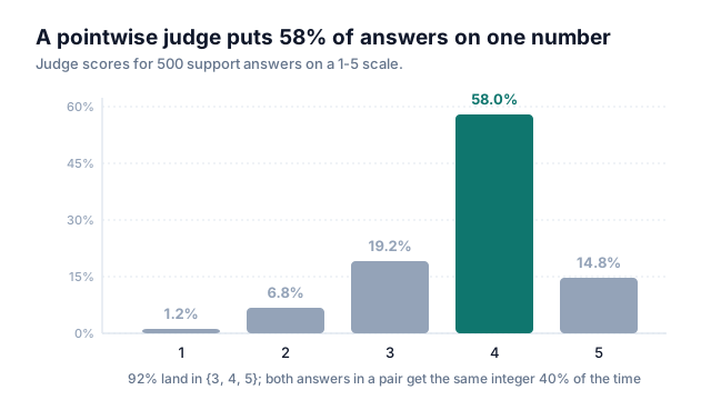
The usual complaint is that small changes get lost in run-to-run noise. That is wrong, and it matters, because it sends you looking for the wrong fix. At n = 500 the standard error on the mean is 0.037, so a shift from 3.78 to 3.88 is nearly three standard errors and perfectly detectable. The problem is resolution: with 58% of answers on the same integer, two answers in a pair come back with the identical score about 40% of the time, and on those pairs the judge has expressed no preference at all. Pairwise also asks the model a question it is better at, and everything from here assumes pairwise, where the judge returns a tie on 28% rather than 40%.
from openai import OpenAI

client = OpenAI()

def judge_pairwise(question, answer_a, answer_b, model):
    """Returns 'A', 'B', 'TIE', or None when the verdict line is missing."""
    prompt = PAIRWISE_TEMPLATE.format(q=question, a=answer_a, b=answer_b)
    resp = client.chat.completions.create(
        model=model,                       # a dated snapshot, never a floating alias
        temperature=0,
        messages=[{"role": "user", "content": prompt}],
    )
    return parse_verdict(resp.choices[0].message.content)
That None earns its place. Over the 1,000 verdicts behind this post, 8 came
back without a parseable verdict line, 6 malformed and 2 refusals on questions the
judge decided were sensitive; one retry cleared 5 of them and 3 were counted as
ties. That is 0.3% of the run, small enough to ignore but worth logging anyway,
because it turns out to be the earliest drift signal in the pipeline. Temperature
0 does not make any of this deterministic either. OpenAI
documents chat completions as non-deterministic by default,
describes seed as a best-effort feature with determinism explicitly not
guaranteed, and the seed and system_fingerprint fields now carry a deprecated
badge on Chat Completions and do not exist on the Responses API at all, so plan
for a judge that answers slightly differently on Tuesday.
The judge has a favourite slot
Show a pairwise judge two answers as (A, B), then again as (B, A), and a fair
judge flips its pick. Mine kept the same slot often enough to matter, which is
measurable in two lines of bookkeeping over the same pairs run twice.
def position_bias(pairs, model):
    """Order-dependence, and the share of decided verdicts that went to slot 1."""
    order_dependent = slot1 = decided = 0
    for q, a, b in pairs:
        v1 = judge_pairwise(q, a, b, model)   # candidate a in slot 1
        v2 = judge_pairwise(q, b, a, model)   # candidate a in slot 2
        mirrored = {v1, v2} == {"A", "B"}     # the judge named the same answer twice
        order_dependent += not (mirrored or v1 == v2 == "TIE")
        for v in (v1, v2):
            if v in ("A", "B"):
                decided += 1
                slot1 += v == "A"
    return order_dependent / len(pairs), slot1 / decided
The mirror test is the whole thing. If the judge names the same physical answer in
both orders the verdicts read A then B, which is why the set comparison and
not an equality is what you want.
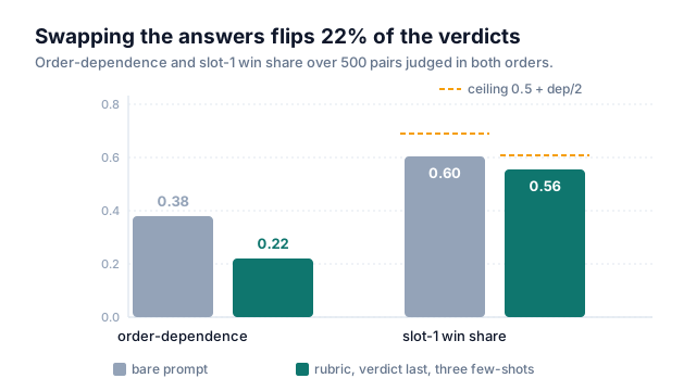
On the bare prompt the judge changed its answer on 38% of pairs when the only thing I changed was the order, and slot 1 took 60% of the decided verdicts. Those two numbers are not independent, and the relationship is worth carrying around because it catches fabricated eval numbers instantly. An order-dependent pair contributes either two slot-1 wins or none; a consistent pair contributes exactly one. So the slot-1 share can never exceed 0.5 plus half the order-dependence rate, which at 38% order-dependence puts the ceiling at 0.69, and any write-up claiming 71% slot-1 alongside 41% order-dependence has one of the two numbers wrong. Published figures land in the same range: MT-Bench reports GPT-4 giving consistent verdicts on 65% of swapped pairs, so 35% order-dependent, rising to 77.5% with few-shot judging. Their test is harder than mine by construction, since the two answers are near-identical samples from one model, so treat 35% as a worst case and 22% as what a tuned prompt on visibly different answers looks like.
Length and family, in log-odds
Length bias hides better than position bias because it lines up with something real, since longer answers are sometimes better. The question is whether length still predicts the verdict once you hold the human label fixed, which is a regression and not a correlation.
I fit the judge’s choice on the holdout against the thing I want plus the nuisances I do not. Position appears as a regressor here because the fit runs on both presentation orders, 1,000 rows from 500 pairs.
import statsmodels.formula.api as smf

m = smf.logit(
    "judge_picks_a ~ human_pref + delta_len_100tok + first_slot + same_family",
    data=df,                               # 1,000 rows: 500 pairs x 2 orders
).fit(disp=0)
print(m.params)                            # log-odds
print(m.get_margeff(at="overall").summary()) # percentage points, easier to argue about| Term | log-odds | effect on the judge’s pick |
|---|---|---|
| human preference | 2.98 | +39.9 points |
| answer-length gap, per 100 tokens | 0.30 | +4.1 points |
| presented first | 0.40 | +5.3 points |
| same model family as the judge | 0.54 | +7.3 points |
Real quality dominates, which is the reassuring part, though a hundred extra tokens buying four points is tolerable in a training signal and corrosive in an automated gate, where it means a short correct answer loses to a padded one more often than it should.
This model does not give you a debiased verdict. Producing one means predicting
with human_pref in the equation, and human_pref is the thing you lack
everywhere outside the holdout, so it is a bias quantifier, good for telling
someone exactly how much the judge pays for verbosity and useless as a correction
layer.
Length-controlled AlpacaEval shows what you
can have without human labels: model the auto-annotator’s own preferences on
observable mediators, then report the win rate that would have been seen at equal
output length. That is a counterfactual aggregate, which a leaderboard can use and
a merge gate cannot.
The same-family coefficient is a property of my candidate mix, not a constant. The self-recognition work finds GPT-4 preferring its own generations at 0.705 on one summarisation set and 0.912 on another, so the size of this effect moves a lot with the data. MT-Bench’s own authors decline to conclude that self-enhancement bias exists at all, given how small and noisy the differences were. Measure it on your mix; do not import a number.
The judge rewards sounding sure
The first three biases are easy to catch once you look. The one that does real damage is that the judge rewards confidence and agreement whether or not the answer is right. Two answers to “what’s my deductible?”:
A. “Your deductible is $1,500.”
B. “It looks like $1,500 on your current plan, though that can change mid-year if you switch tiers. Worth confirming in your benefits portal.”
A sounds more certain, but B is more honest, and in a regulated setting B is the one you want to ship. The plain judge, however, picks A most of the time, reading hedging as weakness and a firm wrong answer as strength, so an automated gate left on its defaults pushes the system away from calibrated uncertainty in exactly the domains where a confident wrong answer is the worst outcome available. Reading the judge’s own reasoning on the pairs it got wrong is the fastest way to build a rubric against that. Two from my file:
Q: “Can I expense a business-class flight?” A (reviewer’s pick): “No. The policy caps international flights at economy unless the leg is over 8 hours.” B: “Great question! Travel policies vary, and there are several factors to consider. Generally, many companies allow business class in certain circumstances… (180 more words)” Judge: picked B, “more thorough and helpful.” B never answered the question.
Q: “Is this transaction fraudulent?” A: “Yes, this is definitely fraud.” B (reviewer’s pick): “Two signals are unusual (geo-velocity, amount), but device and merchant check out. I’d flag for review, not auto-decline.” Judge: picked A, “clear and decisive.” Calibration was the entire job on that question.
I keep adding to that file, and rubric version 3 came out of it. The criteria-drift finding describes what happened to me exactly: you need criteria to grade outputs, and grading outputs is how you discover the criteria, which means the rubric is downstream of the errors you have already seen and cannot anticipate the ones you haven’t.
Cheap gains before you buy extra calls
The cheapest gains are in the prompt, before you spend a single extra call. A rubric that spells out what grounded and helpful mean here and names what to penalise, reasoning before the verdict with the winner on the last line so the judge cannot blurt a letter and argue backward, and three few-shot examples labelled by the same reviewer whose judgment the judge is supposed to match.
You are comparing two answers to a customer's question. Judge only on:
  (1) groundedness: is every claim supported by the provided context?
  (2) correctness: does it actually answer the question asked?
  (3) calibration: does confidence match the evidence? Penalize a confident
      wrong answer MORE than an honest "I'm not sure."
Do NOT reward length, formatting, or a friendly tone on their own.

First write 2-3 sentences comparing the answers on these axes.
Then, on the LAST line, output exactly: WINNER: A   or   WINNER: B   or   TIE.

<three labeled examples follow>
That took agreement from 66.0% to 72.0% and order-dependence from 38% to 22%. It also introduced a problem I did not see until the generator changed under it. Version 3 exists because I read the judge’s mistakes, and those mistakes were made on outputs from one particular candidate model, so the rubric is fitted to that model’s tics: the opening flourish, the stacked hedge, the preamble before the answer. When we swapped the answer generator, several clauses stopped binding, because there was no friendly tone left to decline to reward, and judge agreement moved without a byte of the judge changing. A rubric written after reading outputs is in-sample on the model that produced them. I have no clean fix, only a habit: re-read it clause by clause when the generator changes, and ask which failure each clause was written against and whether that failure still happens.
No prompt kills position bias, so the next call buys symmetry instead of intelligence:
flowchart TD
  P["Pair (X, Y)"] --> O1["Judge order (X, Y)"]
  P --> O2["Judge order (Y, X)"]
  O1 --> C{Same answer<br/>named twice?}
  O2 --> C
  C -->|yes| K["Keep the verdict"]
  C -->|no| F["Tie, and into<br/>the labelling queue"]
  style K fill:#0f766e22,stroke:#0f766e
  style F fill:#f59e0b22,stroke:#b45309
def robust_verdict(q, a, b, model):
    v1 = judge_pairwise(q, a, b, model)
    v2 = judge_pairwise(q, b, a, model)     # swapped
    if v1 == "A" and v2 == "B":             # both point at a
        return "a"
    if v1 == "B" and v2 == "A":             # both point at b
        return "b"
    return "tie"                            # order moved it, so do not trust it
Position bias cancels by symmetry here, exactly. What comes out the other side is 360 decided pairs and 140 ties, and those 140 are the same pairs that were order-dependent plus the ones the judge called a tie in both orders. Hold on to that number; it comes back twice.
| Configuration | agreement | Cohen’s kappa |
|---|---|---|
| bare prompt, one order | 66.0% | 0.42 |
| rubric, verdict last, few-shot | 72.0% | 0.53 |
| the same, plus swap | 77.4% | 0.65 |
| two humans | 86.8% | 0.79 |
Watch kappa rather than raw agreement, and watch it against the last row. The judge recovers 83% of the kappa two senior reviewers reach with each other, and the remaining gap is the honest budget for further work.
How many labels you actually have to buy
Labelling is the expensive thing the judge was supposed to save you, so the question is how small the random holdout can be, and the way to answer it is to bootstrap the kappa and watch what the interval does as you shrink the set.
import numpy as np
from sklearn.metrics import cohen_kappa_score

LABELS = ["a", "b", "tie"]

def kappa_ci(human, machine, n_boot=3000, alpha=0.05):
    human, machine = np.asarray(human), np.asarray(machine)
    stats = np.empty(n_boot)
    for i in range(n_boot):
        idx = np.random.randint(0, len(human), len(human))
        stats[i] = cohen_kappa_score(human[idx], machine[idx], labels=LABELS)
    lo, hi = np.percentile(stats, [100 * alpha / 2, 100 * (1 - alpha / 2)])
    return float(stats.mean()), float(lo), float(hi)
Passing labels= is not optional. A bootstrap resample of a 500-pair holdout will
sometimes contain no ties at all, and without the explicit label list the kappa
for that draw is computed over a two-category space, which shifts the
chance-agreement term and biases the whole interval without raising anything. In
scikit-learn 1.9 the argument became keyword-only, and the two positional
arguments are still y1 and y2, not the y_true and y_pred used elsewhere in
sklearn.metrics.
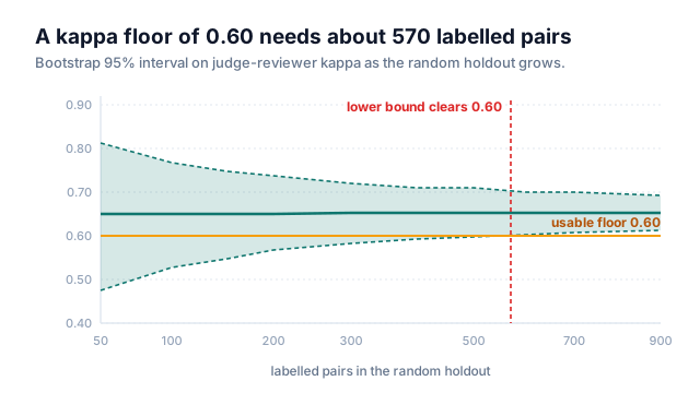
At 100 pairs the interval is [0.53, 0.77], which tells you the judge is not
random and nothing else, and at 500 it is [0.598, 0.709]. The lower bound reaches
the usable line of 0.60 somewhere around 570 pairs, and that is the number that
changed how I gate, because a CI test that reads assert lo >= 0.6 demands a
holdout of roughly 570 double-checked labels before it can ever pass, which for
most teams costs more than the judge saves. So gate on the point estimate with a
stated holdout size, and put the expensive guarantee somewhere it is affordable,
which is the drift test further down.
Then spend the rest of the budget on the 140 ties. Those are the pairs where the swap disagreed with itself, which makes them the highest-uncertainty items in the set and a ready-made queue, and none of them may go anywhere near a kappa, an AC1, or a PPI rectifier, because a set selected for being hard is not a sample of anything.
Which agreement number is honest
When one outcome dominates, kappa sits near zero even though the two raters agree almost every time, because chance agreement under a lopsided distribution is high and the correction eats the real agreement. This is the prevalence problem, and the usual advice is to report Gwet’s AC1 instead. On the pairwise holdout that advice buys almost nothing, and the two columns below are why.
| Coefficient | pairwise pick | groundedness flag |
|---|---|---|
| raw agreement | 0.774 | 0.950 |
| Cohen’s kappa | 0.653 | 0.640 |
| Gwet’s AC1 | 0.667 | 0.942 |
| Krippendorff’s alpha, nominal | 0.650 | 0.640 |
Same 500 pairs, same two raters, same afternoon. The left column is the a/b/tie preference, where the marginals are 45/40/15 and chance agreement lands at 0.35, close to the 0.33 of a uniform three-way split. Kappa and AC1 differ by 0.014 and you can report either. The right column is a binary groundedness flag over the same answers, where 92% pass, chance agreement under kappa’s model is 0.86, and the two coefficients differ by 0.30. Reporting kappa there says the judge is mediocre; reporting AC1 says it is excellent; the honest reading is that at 95% agreement on a 92%-prevalent label, kappa has very little signal left to work with.
Which coefficient you owe the reader is not a statistics preference. It is decided by the marginal balance of the label you happen to be gating on, and that label was defined by whoever wrote the product requirement, so a team that changes “is this grounded” from a binary flag to a three-way severity rating has changed which reliability coefficient is meaningful, and nobody in that conversation will mention it.
Prevalence is the failure everyone names. There is a second one running the other
way, and the swap from the previous section walks into it. Chance agreement is the
inner product of the two raters’ marginals, so moving judge mass into the category
the reviewer uses least pulls pe down and pushes kappa up with no change in how
often the judge is right, and swap-and-aggregate does exactly that, lifting
verdicts out of a and b and dropping them into tie, the reviewer’s rarest label.
Raw agreement rose too, 72.0% to 77.4%, so most of the gain is real, but the kappa
move from 0.53 to 0.65 reads as the bigger win and some of that extra is the
marginal shift and not the judge. It also means the swap isn’t portable: what a
converted tie earns you depends on how often your reviewers call ties at all, and
that is set by the annotation guideline, so under one that says pick one, no ties,
every verdict the swap converts lands off the diagonal.
from irrCAC.raw import CAC

cac = CAC(ratings_df)                        # rows = pairs, columns = {reviewer, judge}
est = cac.gwet()["est"]
print(est["coefficient_value"], est["pa"], est["pe"])   # 0.6665  0.7740  0.3223
alpha = cac.krippendorff()["est"]["coefficient_value"]
The est dict carries pa and pe alongside the coefficient, and printing both
is how you catch this without thinking about it: when pe is 0.86 you are in the
prevalence regime and when it is 0.32 you are not.
CAC also exposes conger(), which
for two raters returns Cohen’s kappa exactly, and reproducing your own kappa
through it is a cheap check that the dataframe is oriented the way the library
expects.
From win rates to abilities
A raw win rate throws information away. If A beats B 55% of the time and B beats C 60%, and you also ran A against C, those three numbers constrain each other. Bradley-Terry gives every system a latent ability and makes the probability that i beats j the logistic of their gap:
You fit it with logistic regression on the pairwise outcomes, which is also how the Chatbot Arena ratings are computed:
import numpy as np
from sklearn.linear_model import LogisticRegression

def bradley_terry(comparisons, n_systems):
    """comparisons: (i, j, i_won) triples. Sign by SLOT, not by outcome."""
    X = np.zeros((len(comparisons), n_systems))
    y = np.zeros(len(comparisons), dtype=int)
    for r, (i, j, i_won) in enumerate(comparisons):
        X[r, i], X[r, j] = 1.0, -1.0
        y[r] = i_won
    lr = LogisticRegression(fit_intercept=False, C=1e4, max_iter=1000).fit(X, y)
    theta = lr.coef_[0]
    return theta - theta.mean()              # abilities are relative, so centre them
The design matrix has to be signed by slot and the label has to carry the outcome.
Signing by winner instead, so the winner’s column is always +1, makes every
label a 1, and
LogisticRegression.fit
raises on the spot: “This solver needs samples of at least 2 classes in the data,
but the data contains only one class”. Two other details matter. C=1e4 is there
to make the regularisation negligible, because the default C=1.0 shrinks
abilities toward zero and compresses the ranking you are trying to read. And
centring does real work here, because only differences are identified, so an
uncentred fit gives you numbers that move between runs for no reason.
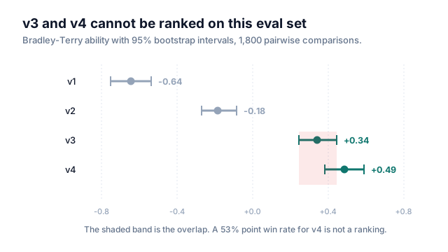
Refit on a thousand bootstrap resamples of the comparisons and you get a ranking with error bars. v3 at +0.34 and v4 at +0.49 have overlapping intervals, so on this eval set they are not distinguishable, whatever the point win rate says. The fitted gap implies v4 beats v3 53.6% of the time, which is where the head-to-head number in the next section comes from and a useful consistency check on the fit.
Ties need care. Plain Bradley-Terry has no tie outcome, and 140 of my 500 pairs are ties, so dropping them discards 28% of the data and biases what remains toward easy pairs. The Davidson extension adds a tie parameter and a three-way likelihood over {i wins, j wins, tie}, which is what you want when ties are this common. Scoring a tie as half a win to each side is the convention you will find in most implementations, but it is not the same model, since it assumes ties carry no information about how close the systems are, which is the one thing you were hoping to learn from them. Elo, meanwhile, is an online approximation of Bradley-Terry whose ratings depend on the order the matches arrived in. For a fixed eval set you hold every game at once, so fit the full model and skip the path dependence.
Is the win real
The release comparison ran 1,800 pairs and the new system won 53.0% of them. That feels safe, but two things break the naive test. The first is that the pairs are not independent: my 1,800 pairs come from 240 distinct customer intents, roughly seven paraphrases of the same underlying question each, and answers to near-duplicate questions succeed and fail together, which puts the effective sample size closer to the number of intents than the number of pairs. So the bootstrap has to resample intents rather than pairs.
import numpy as np

def clustered_win_ci(pairs_by_query, n_boot=4000):
    queries = list(pairs_by_query)
    rates = np.empty(n_boot)
    for i in range(n_boot):
        picked = np.random.randint(0, len(queries), len(queries))
        wins = [p.new_won for k in picked for p in pairs_by_query[queries[k]]]
        rates[i] = np.mean(wins)
    return np.percentile(rates, [2.5, 97.5])
Resampling pairs gave a 95% interval of [50.8%, 55.3%], which matches the binomial interval to a tenth of a point, as it must. The intent-clustered bootstrap widened it to [48.6%, 57.1%]. The realised intra-cluster correlation was 0.35 and the design effect 3.6, so the honest interval is about 1.8 times wider than the naive one, and it straddles 50%. The win I was ready to announce was not distinguishable from nothing, and the naive interval had hidden that behind a number that looked precise.
It also explains why some published win rates cannot be right. A binomial 95% interval of [51%, 55%] requires about 2,400 pairs; quoted alongside n = 500 it is off by a factor of five, and the naive interval there already straddles 50% before anyone reaches for clustering.
The second problem is running many comparisons. Ten prompt variants against a baseline at alpha 0.05 give roughly a 40% chance that at least one wins by luck, so what you want is control of the false discovery rate rather than of any individual test.
from statsmodels.stats.multitest import multipletests

reject, p_adj, _, _ = multipletests(pvals, alpha=0.05, method="fdr_bh")
On my ten variants, five cleared 0.05 raw and three survived Benjamini-Hochberg.
Note that
multipletests
defaults to method="hs", Holm-Sidak, which controls the family-wise error rate
and is considerably more conservative than what you want when screening variants.
The method argument decides which of the two guarantees you get, and it is not the
kind of default you notice leaving in place.
The gate that grades its own optimizer
Somewhere in the second month the judge picked up a second job. We were already sampling four candidate answers per question and shipping whichever one the judge liked best, and we were gating the release on the judge’s win rate. Those look like two controls, but they are one check run twice. Best-of-n against a judge moves the output distribution toward whatever that judge over-rewards, and then the gate asks the same judge whether the move was an improvement. It says yes. The scaling laws for reward-model overoptimization are the general shape: push far enough against a proxy and the proxy score keeps climbing while the thing it stands in for turns over.
Nothing about the symptom looks like a fault. Judge win rate climbs release over release while kappa on the frozen holdout and the human win rate on the release set both sit still. What I run now keeps the roles apart: the selection judge and the gate judge are different families with different prompts, and the gate judge never scores a candidate that was chosen by it. That costs a second validation holdout, since the gate judge needs its own ceiling and its own drift test.
Where prediction-powered inference stops helping
Prediction-powered inference combines a large judge-scored set with a small human-scored one into a confidence interval on the true, human-defined metric, with valid coverage instead of a hope, and usually it is tighter than the human-only interval. The estimator is small: compute the metric on the unlabelled set the judge scored, then subtract the judge’s systematic error measured on the labelled subset.
import numpy as np

def ppi_mean(f_unlabeled, f_labeled, y_labeled, z=1.96):
    """f_unlabeled must be DISJOINT from f_labeled, or the rectifier is wrong."""
    theta = f_unlabeled.mean() - (f_labeled - y_labeled).mean()
    se = np.sqrt((f_labeled - y_labeled).var(ddof=1) / len(y_labeled)
                 + f_unlabeled.var(ddof=1) / len(f_unlabeled))
    return theta, theta - z * se, theta + z * se
The disjointness in that docstring is load-bearing. The two variance terms add instead of combining through a covariance precisely because the samples are independent, so pooling the labelled rows into the large set breaks the interval while leaving the point estimate looking fine.
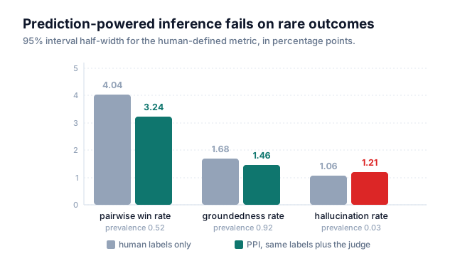
Now the part that surprised me. Read the standard error and the condition for PPI to help falls straight out of it: the method beats the human-only interval when the variance of the judge’s error is smaller than the variance of the outcome itself. Here are three metrics from the same run, which is where I stopped assuming it always helps.
| Metric | prevalence | human labels only | with PPI |
|---|---|---|---|
| pairwise win rate | 0.52 | ±4.04 points | ±3.24 points |
| groundedness rate | 0.92 | ±1.68 points | ±1.46 points |
| hallucination rate | 0.03 | ±1.06 points | ±1.21 points |
The hallucination rate is the interesting row. Judge-human agreement on that label is 96.5%, the highest anywhere in this post, yet PPI still made the interval 14% wider. A 3% base rate leaves the outcome variance at 0.029, while a 3.5% disagreement rate puts the rectifier variance at 0.035, and once the rectifier loses that comparison you are better off ignoring the judge. Rarity, not inaccuracy, is what breaks it, which means the technique for stretching scarce labels stops working exactly where positives are scarcest and you want it most.
The 500 human labels behind the pairwise row bought the precision of about 780, which is a real saving and nowhere near the halving you sometimes see claimed. At 77% agreement halving the interval is arithmetically out of reach; you would need the disagreement rate down near 2%. The power-tuned variant is worth knowing about here, since it fits a coefficient on the judge term and asymptotically dominates the classical estimator, which means the rare-event row above degrades to “no worse than human-only” instead of actively hurting.
Watching for drift without paying for it
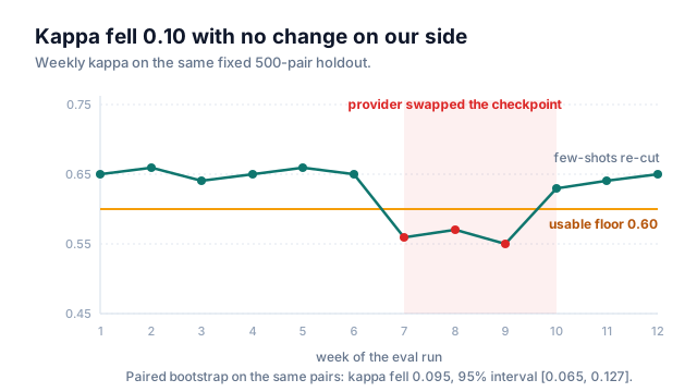
You validate all of this once and it holds. Kappa 0.65, swap-corrected, the ceiling in sight. Then it moves, and three separate things move it. The provider replaces the checkpoint behind a model name. You edit the judge prompt, a small wording change, and forget that it reopens the whole validation. Or your traffic shifts until the holdout stops resembling production. From the outside those look identical, and the dashboard keeps printing clean numbers that mean a little less each week.
The first two are watchable. Pin the dated model snapshot instead of a floating alias and a provider swap becomes something you accepted on a day you know about. The prompt is the one people miss, so treat the judge as an artifact and not a call: the tuple of model snapshot, prompt, rubric version, and few-shots. Hash it, version it, and rerun the holdout whenever the hash moves:
import hashlib, json

def judge_fingerprint(cfg: dict) -> str:
    blob = json.dumps(cfg, sort_keys=True).encode()
    return hashlib.sha256(blob).hexdigest()[:12]

JUDGE = {"model": "gpt-4o-2024-11-20",      # dated snapshot, so a swap is your decision
         "prompt": PAIRWISE_TEMPLATE,
         "rubric_version": 3,
         "n_fewshot": 3}
That fingerprint has a hole in it and it took me two quarters to find. It covers the judge but says nothing about the population the judge was validated against, so replacing the answer generator invalidates the holdout without moving the hash by a bit. I stamp the generator’s version onto the holdout record too now, and a change there is a reason to relabel.
Now the part that makes this affordable. Detecting drift is a much cheaper statistical question than establishing an absolute floor, because the same fixed pairs make the comparison paired. When the checkpoint moved under me, kappa went from 0.653 to 0.557, and the two independent bootstrap intervals were [0.598, 0.706] and [0.501, 0.614], which overlap, so an unpaired read of those two numbers says nothing happened. Resampling the same pair indices for both runs and bootstrapping the difference instead gives a drop of 0.095 with a 95% interval of [0.065, 0.127].
import numpy as np
from sklearn.metrics import cohen_kappa_score
from statsmodels.stats.contingency_tables import mcnemar

LABELS = ["a", "b", "tie"]

def kappa_drop_ci(human, before, after, n_boot=3000):
    """Same holdout, two judge versions. Resample pairs ONCE per draw."""
    human, before, after = map(np.asarray, (human, before, after))
    d = np.empty(n_boot)
    for i in range(n_boot):
        idx = np.random.randint(0, len(human), len(human))
        d[i] = (cohen_kappa_score(human[idx], before[idx], labels=LABELS)
                - cohen_kappa_score(human[idx], after[idx], labels=LABELS))
    return float(d.mean()), *np.percentile(d, [2.5, 97.5])

def agreement_shift_p(human, before, after):
    """b = agreed then disagreed, c = disagreed then agreed."""
    ok_b, ok_a = np.asarray(before) == human, np.asarray(after) == human
    table = [[int((ok_b & ok_a).sum()), int((ok_b & ~ok_a).sum())],
             [int((~ok_b & ok_a).sum()), int((~ok_b & ~ok_a).sum())]]
    return mcnemar(table, exact=True).pvalue
The McNemar test on the same data gives p = 2e-5 off 44 pairs that stopped agreeing against 12 that started. So the alarm in CI is the paired one, on a holdout you never rotate, and the absolute kappa floor becomes something you check once a quarter when you can afford fresh labels. Most eval pipelines have this backwards and assert the expensive claim on every run.
Which leaves the third cause, invisible for exactly the reason the paired test is cheap: what makes it work is that the holdout never moves, and a set that never moves cannot tell you traffic walked away from it. What is watchable without spending a label is the judge’s own output distribution, the share of a, b and tie it returns on live traffic against the share it returns on the holdout. When the production tie rate pulls away from the holdout’s, either the traffic got harder or the judge got shakier, and both are reasons to go and buy labels.
The parse-failure counter earns its place here too. When the checkpoint moved, the unparseable rate went from 0.3% to 1.9% in the same run that kappa dropped, and it is one integer to log against 500 pairs of human labelling. I would not gate on it, since one run is one run and I have no idea whether the two move together in general, but it is free and it fired first.
What the calls cost
Swapping doubles your judge calls and a three-judge panel triples that again. At eval scale the token volume is the whole bill: one single-order pass over 1,800 pairs is about 2.5M input tokens at roughly 1,400 tokens per comparison, a swapped pass is 5.0M, and a swapped three-judge panel is 15.1M.
| Setup | calls per pair | agreement | kappa |
|---|---|---|---|
| small model, one order | 1 | 66.4% | 0.44 |
| small model, swapped | 2 | 71.4% | 0.57 |
| strong model, one order | 1 | 72.0% | 0.53 |
| strong model, swapped | 2 | 77.4% | 0.65 |
| three judges, mixed families, swapped | 6 | 80.6% | 0.70 |
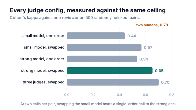
The two-call rows are the ones to compare, because they cost the same number of round trips. Swapping the small model reaches 0.57 at a small fraction of the price per token, whereas a single-order call to the strong model reaches 0.53. Buy the second call before you buy the bigger model. The panel buys another 0.05 of kappa for three times the calls, mostly by cancelling self-preference across families, and it is a release-gate expense rather than a per-PR one.
What I run now is the swapped small judge on every pull request to catch regressions, the strong swapped judge on the release gate, and the panel only when a result is going to be quoted outside the team.
The bill is not the binding constraint though. You cannot judge everything, so you sample, and the moment you sample by anything other than a coin you have put back the problem the random holdout was built to remove. Judging the sessions that got a thumbs-down, or the ones a human escalated, buys a reading on the hard tail and an estimate of nothing. So the sampling probability gets written next to the verdict. A known unequal probability is recoverable, and there are PPI intervals for weighted, stratified and clustered labelled samples that will take one. An unrecorded probability is recoverable by nothing, and “we judged the interesting ones” is unrecorded by construction.
When not to use a judge at all
Often the right answer is not to use one. If the thing you are checking is checkable, check it: exact match, a JSON schema, a unit test, running the generated SQL and diffing the rows. Those do not drift, do not develop preferences, and do not need a 500-pair holdout before you can trust them, so save the judge for what is irreducibly subjective. Something like half the LLM-as-judge setups I have looked at were grading things a five-line assertion could have graded for free, and paying for a biased, drifting ruler on top of it.
The working setup
- Pairwise for anything subjective, deterministic checks for anything else.
- A random holdout of 500 pairs, double-labelled, reserved before any active selection starts, and never rotated. It is the only pool a measurement may touch.
- The prompt first: a real rubric, reasoning before the verdict, few-shot examples from the reviewer I am matching.
- Always swap. A single-order verdict is a weighted coin and the second call is cheaper than a bigger model.
- Report kappa next to the human-human ceiling, always. Report AC1 as well when
the label’s chance agreement runs above about 0.6, and print
paandpeso the reason is visible. - Bradley-Terry with bootstrap intervals for rankings, Davidson when ties are more than a few percent, and no ranking between two systems whose intervals overlap.
- Query-clustered bootstrap for every difference, and false-discovery control the moment I compare more than two candidates.
- PPI where the outcome is common and the judge is close, and human labels alone where the outcome is rare.
- The judge hashed as (snapshot, prompt, rubric, few-shots), the answer generator’s version stamped alongside it, a paired drift test against the fixed holdout on every run, and the absolute kappa floor rechecked quarterly.
- The rubric re-read clause by clause whenever the generator changes, and the selection judge kept apart from the gate judge so the gate is not grading its own optimizer.
- The sampling probability recorded next to every production verdict, because an unknown one cannot be weighted back out later.
- The parse-failure rate and the judge’s a/b/tie shares on live traffic logged as first-class metrics.
All of it is the ordinary care you would give any measuring instrument you had not calibrated. It only feels strange applied to a model, because a model answers back fluently enough that checking it feels rude. Worth doing anyway, given that this particular instrument is already deciding what ships.